Tensors
Tensor = container
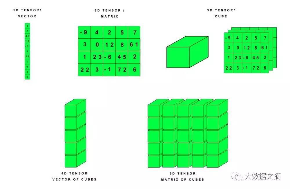
Tensors are the foundation everything in modern machine learning sits on. At its core a tensor is just a container — usually of numbers, occasionally of strings, though that’s rarer. Think of it as a bucket of numbers.
A 0-D tensor is a scalar; a 1-D tensor is a vector; a 2-D tensor is a matrix; a 3-D tensor (and up) is what you use for shared data storage — things like color images.
One-hot vectors
One-hot encoding is used for categorical labels. For example, (cat, dog, mouse) maps to (1,0,0) for cat, (0,1,0) for dog, and so on. Encoding discrete features this way makes distance calculations between features much more sensible.
The softmax function
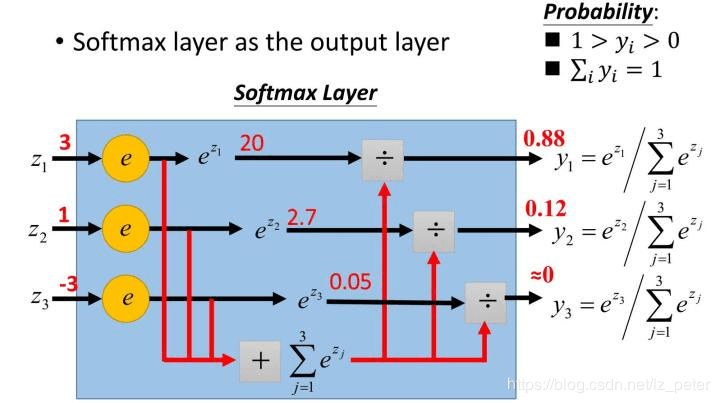
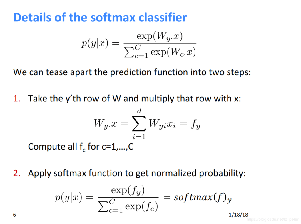
Softmax does two things: it runs the model’s raw scores through an exponential function so they all come out non-negative, and then it normalizes them so all the resulting probabilities add up to 1.
Cross-entropy
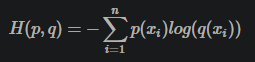
For single-label multi-class classification, p(x) is the ground-truth label — with one-hot encoding this is just 0 or 1 — and q(x) is the predicted probability for that class. Using cross-entropy as the loss function, the smaller the value, the closer the model’s predictions are to reality.
In single-label multi-class problems, the probabilities across all classes sum to 1. In multi-label binary classification they don’t — cross-entropy there is computed per class (as a binary decision), and then you sum the binary cross-entropy across classes for a given sample.
Euclidean space
Euclidean space is just the formal, generalized version of the physical space we’re used to — extended from n ≤ 3 dimensions to any finite n dimensions.
Euclidean geometry is the plane and solid geometry you learned in school — where, notably, parallel lines stay the same distance apart everywhere.
The geometry you learn in school is normally 2D or 3D (which is why cosine similarity, distances between points, and inner products all get introduced in low-dimensional space first). Once you generalize the rules you learned in those low-dimensional spaces to any finite n dimensions, spaces that satisfy those definitions are what we call Euclidean space. What Euclidean space really defines is the inner product, distance, and angle — the same concepts from middle school geometry. Once that clicks, the formal math definition makes a lot more sense.
Vanishing and exploding gradients
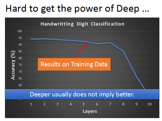
Hidden layers closer to the output have larger gradients, so their parameters update quickly and converge fast.
Hidden layers closer to the input have much smaller gradients, so they update slowly and stay close to their random initial state.
In the four-layer hidden network shown above, the first layer trains almost 100x slower than the fourth!
That’s the vanishing gradient problem. The opposite case — where gradients in earlier layers grow through training and gradients in later layers grow exponentially — is called the exploding gradient problem.
Bottom line: in a deep network, gradients can get pretty unstable.
Batch size
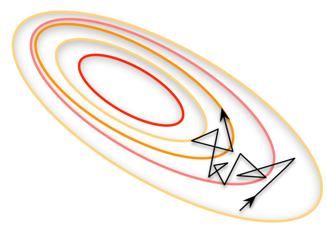
The batch size mainly determines the direction of descent — the bigger the batch, the more accurate that direction.
It comes down to the size of your dataset. When the dataset is small, you can just use the whole thing as your batch, which gives you the most accurate descent direction. When it’s large, a relatively small batch can still get you a global learning rate similar to using the full dataset — so the real trade-off is learning effectiveness versus efficiency versus how much memory your machine actually has, and you want to max out both effectiveness and efficiency at once.
What do you gain from increasing batch size within a reasonable range?
- Better memory utilization, and more efficient parallelization for large matrix multiplications.
- Fewer iterations needed to finish one epoch, so you process the same amount of data faster overall.
- Generally, a larger batch size gives a more accurate descent direction and less training oscillation.
Past a certain point, though, increasing batch size further stops helping efficiency, and the descent direction barely changes anymore.
Learning rate
Pseudocode for gradient descent:
Repeat until convergence: {ωj = ωj − λF(ωj)/ωj}
λ is the learning rate. Too small, and optimization can be painfully slow; too large, and you risk overshooting the optimum and converging to a local minimum instead.
For more on picking a good learning rate, adjusting it dynamically, normalization, etc., see:
How to explain Euclidean space in plain terms? - Zhihu //www.zhihu.com/question/27903807/answer/699570097